Metallurgy with MAGMASOFT: Ductile Iron
About The Ductile Iron Workshop
The Ductile Iron Workshop at Georgia Southern University was developed to bridge the gap between metallurgical theory and practical application. This two-day event provides students with hands-on experience in ductile iron casting, simulation, and microstructural evaluation. By exploring key process variables—such as inoculation rate, pouring temperature and section thickness—participants learn how these factors influence material properties and how simulation tools like MAGMASOFT® can be used to accurately predict real-world outcomes. The workshop equips future engineers with essential skills to connect digital models with physical results and empowers experienced engineers with simulation tools that can expedite their engineering process, fostering a deeper understanding of ductile iron metallurgy.
Purpose
The purpose of the Ductile Iron Workshop is to demonstrate the relationship between process variation and casting properties. By pouring real castings, the trends can be shown with real and simulated data. This case study will focus on 2 of the 4 variables that are set within the scope of the workshop: inoculation rate and sections thickness. The whole workshop explored the impact of two additional variables, pouring temperature and carbon equivalent. However, pouring temperature and carbon equivalent will not be included as variables in this evaluation. The effect on nodule count and hardness will be reported, showing how MAGMASOFT and real life share the same inspiration: metallurgy.
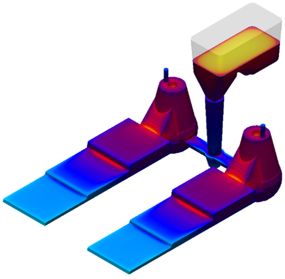
The Casting
A step block was designed to represent 3 families of ductile iron parts. The first step has a thickness of 25mm (~1 inch) and mirrors the threshold where parts start to be defined as “heavy section ductile iron”. Completely opposite, the third step has a thickness of 6mm (~0.25 inch) and represents where parts begin to be considered “thin-walled ductile iron”. The second step has a thickness of 12mm (~0.5 inch) and is similar the average size of ductile iron castings. By having one casting represent all three, the groups can be compared directly with no concern for variation. However, data will be pulled from two step blocks in this study to show how inoculation rate will affect properties across all three sections. Additionally, the increase in inoculation was accomplished with an addition of inoculant in-mold on one cavity of the casting so that concern of variation from mold-to-mold can be reduced to zero.
The Results
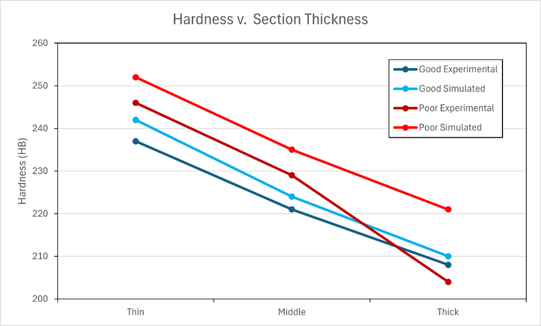
After proper correlation work, the simulated results are remarkably close to the experimental data. The percent difference between the simulated nodule count and the experimental nodule count never exceeds 23% difference and typically hovers around 15%. Additionally, the simulated hardness values are within a 10 HB variation (aside from one value) compared to the experimental values. For context, measuring a single indentation mark from a Brinell hardness test can have the same range in variation and is typically averaged to a mean value.


Plotting the data highlights some interesting trends. For example, the hardness and nodule count go down as the section thickness gets thicker. This is shown in figure 1 and figure 2 by the slope of the lines. The values for good inoculation are plotted in blue and the values for poor inoculation are plotted in red. Additionally, the experimental values are plotted in a darker color than the simulated values. The nodule count recorded from the casting with good inoculation are above the values recorded for poor inoculation in figure 1, showing that inoculation increases the number of nodules in the casting. In contrast, it causes hardness to go down in figure 2 where the blue lines for good inoculation are now below the red lines. So, we can see that nodule count and hardness fluctuate but do not always trend together for each variable considered.

Relationship with DI Metallurgy
The prediction of nodule count in MAGMASOFT® can be broken down to a basic equation. By no extent does this equation encompass all the variables being accounted for in the software, however, it helps to break down some of the theory. N indicates the number of nodules per mm3. “A” and “B” are constants in which A can be determined from user input on metallurgical quality, and ΔT is local supercooling. Utilizing this theory, the software modulates the nodule count in reference to the metallurgical quality of the iron, and in turn can predict the metallurgical and mechanical properties.
Nv = A * ΔTB
In this case study, it is shown that the model is capable of correlating to the nodule count and hardness very well. This is possible because the mechanical properties are determined by the microstructure that is heavily related to the inoculation practice of the foundry. So, nodule count and hardness can be predicted by providing the software with a quantitative value to represent the effectiveness of the inoculation practice in the form of “A”.
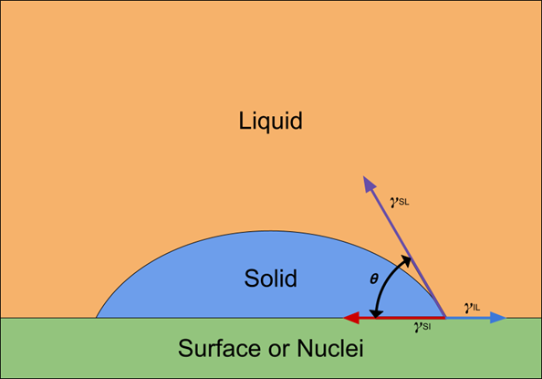
Nodules in ductile iron are formed by carbon latching onto a nucleus and forming a sphere of graphite through a process known as heterogeneous nucleation. Figure 3 is a diagram of how a nucleus acts as a substrate for heterogeneous nucleation. The interfacial energies of the solid-surface (γSI), solid-liquid (γSL), and liquid-surface (γIL) are represented by vectors while the wetting angle (θ) is represented with a curved arrow. The balance of these energies determines the stability of the nucleus to promote solid phase growth. Inoculation provides iron with the nuclei and better inoculation leads to more nuclei, allowing for more opportunities to form graphite. So, the previous equation is related to predicting of the number of nuclei that the iron has the potential to nucleate graphite onto, in relation to metallurgical quality and inoculation.
In addition to forming the nodule, it essentially will localize the carbon in the liquid iron on to points that are 100% carbon. Each nodule can be seen as a high concentration of carbon that will leave the surrounding metal low in carbon, losing carbon to form the nodule. This leads to a structure in the iron, which is low in carbon, ferrite. Ferrite and Graphite are soft structures in the iron compared to the last possible structure, pearlite. So, the microstructure is composed of graphite, ferrite, and pearlite. Inoculation, chemistry, thermodynamics, and kinetics will determine the composition of the iron. By inoculating the iron, the portion of the structure that is graphite and ferrite will increase and lead to lower hardness. Figure 4 is a picture of the microstructure of one of the ductile iron samples in the study. The black spheres are the graphite nodules, and the white ring around each of them is the ferrite formed due to the low carbon zone. The surrounding grey areas are pearlite grains.

1* Callister WD, Rethwisch DG. Materials science and engineering: an introduction. 10th ed. Hoboken, Nj: Wiley; 2018.
 Follow our official Wechat!